05 - Uncertainty quantification

Three drop-in estimators in maldideepkit.uncertainty wrap a fitted classifier and report per-sample uncertainty alongside the usual predictions:

1. Monte Carlo Dropout - stochastic forward passes with dropout layers active. Decomposes total uncertainty into epistemic (model disagreement) and aleatoric (data noise) components (Gal & Ghahramani, 2016; Kendall & Gal, 2017).

2. Laplace approximation - last-layer or full-network Gaussian posterior over the weights, via `laplace-torch <aleximmer/Laplace>`__. Requires the optional uncertainty extra: pip install "maldideepkit[uncertainty]".

3. Split conformal prediction - distribution-free prediction sets with a coverage guarantee. Pure NumPy, no extra deps.

All three return a common UncertaintyResult dataclass, so call sites stay the same when you swap methods.

Uses the MALDI-Kleb-AI dataset cached by notebooks/_demo.py (see notebook 01).

1. Load the demo dataset

import sys, pathlib
sys.path.insert(0, str(pathlib.Path.cwd().parent))  # make notebooks/_demo.py importable
from notebooks._demo import binary_labels, load_maldi_kleb_ai

demo = load_maldi_kleb_ai(antibiotic='Amikacin', verbose=True)
X, y = binary_labels(demo)  # y == 1 for resistant
print(f'X: {X.shape} | prevalence(R): {y.mean():.2%}')

X: (741, 6000) | prevalence(R): 49.80%

2. Train / calibration / test split

We carve the data into three disjoint pieces:

• train - fits the base MaldiMLPClassifier.

• calibration - held out for LaplaceEstimator.calibrate() and ConformalPredictor.calibrate(). MC Dropout needs no calibration set.

• test - never seen during training or calibration; the uncertainty estimates we evaluate below all come from this split.

from sklearn.model_selection import train_test_split

X_tr, X_rest, y_tr, y_rest = train_test_split(
    X, y, test_size=0.40, stratify=y, random_state=0,
)
X_cal, X_te, y_cal, y_te = train_test_split(
    X_rest, y_rest, test_size=0.50, stratify=y_rest, random_state=0,
)
print(f'train: {X_tr.shape[0]} | cal: {X_cal.shape[0]} | test: {X_te.shape[0]}')

train: 444 | cal: 148 | test: 149

3. Fit the base classifier

MaldiMLPClassifier ships with dropout layers on by default, so the same fitted model serves all three uncertainty estimators below. We add calibrate_temperature=True to keep the softmax probabilities well-scaled before any post-hoc calibration kicks in.

from maldideepkit import MaldiMLPClassifier

clf = MaldiMLPClassifier(
    epochs=40,
    batch_size=32,
    calibrate_temperature=True,
    random_state=0,
).fit(X_tr, y_tr)

print(f'test accuracy: {clf.score(X_te, y_te):.3f}')
print(f'fitted temperature: {clf.temperature_:.3f}')

test accuracy: 0.779
fitted temperature: 1.293

4. Monte Carlo Dropout

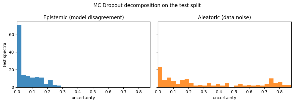
Run n_samples=50 stochastic forward passes through clf.model_ with dropout layers kept in training mode. The variance of the resulting softmax distribution is interpreted as epistemic uncertainty (model disagreement); the mean of the per-pass entropies is interpreted as aleatoric uncertainty (data noise).

No calibration step is needed - MC Dropout reuses the dropout stochasticity baked into the fitted model.

import numpy as np
from maldideepkit.uncertainty import MCDropoutEstimator

mc = MCDropoutEstimator(clf, n_samples=50)
mc_result = mc.predict_with_uncertainty(X_te)

print(f'method:        {mc_result.method}')
print(f'predictions:   {mc_result.predictions.shape}')
print(f'proba_mean:    {mc_result.proba_mean.shape}')
print(f'total H:       mean={mc_result.uncertainty.mean():.3f}  '
      f'p10={np.quantile(mc_result.uncertainty, 0.1):.3f}  '
      f'p90={np.quantile(mc_result.uncertainty, 0.9):.3f}')
print(f'epistemic:     mean={mc_result.epistemic.mean():.3f}')
print(f'aleatoric:     mean={mc_result.aleatoric.mean():.3f}')

method:        mc_dropout
predictions:   (149,)
proba_mean:    (149, 2)
total H:       mean=0.411  p10=0.021  p90=0.960
epistemic:     mean=0.070
aleatoric:     mean=0.340

Plot the epistemic / aleatoric decomposition. A spectrum with high epistemic uncertainty is one the model has not seen enough similar examples of - a candidate for active labelling. High aleatoric uncertainty signals genuine label ambiguity that more data will not resolve.

import matplotlib.pyplot as plt
import numpy as np

x_max = float(np.maximum(mc_result.epistemic.max(), mc_result.aleatoric.max()))
bins = np.linspace(0.0, x_max, 31)

fig, axes = plt.subplots(1, 2, figsize=(10, 3.5), sharex=True, sharey=True)
axes[0].hist(mc_result.epistemic, bins=bins, color='C0', alpha=0.85)
axes[0].set_title('Epistemic (model disagreement)')
axes[0].set_xlabel('uncertainty')
axes[0].set_ylabel('test spectra')
axes[1].hist(mc_result.aleatoric, bins=bins, color='C1', alpha=0.85)
axes[1].set_title('Aleatoric (data noise)')
axes[1].set_xlabel('uncertainty')
axes[0].set_xlim(0.0, x_max)
fig.suptitle('MC Dropout decomposition on the test split')
fig.tight_layout()
plt.show()

5. Split conformal prediction

ConformalPredictor learns a single quantile on the calibration split, then returns a prediction set per test spectrum that contains the true class with marginal probability \(\geq 1 - \alpha\). With alpha=0.1 we target 90 % coverage.

Per-sample uncertainty is the prediction set size normalised by n_classes: 1 / n_classes for a confident singleton, 1.0 when every class is included.

from maldideepkit.uncertainty import ConformalPredictor

cp = ConformalPredictor(clf, alpha=0.10).calibrate(X_cal, y_cal)
cp_result = cp.predict_with_uncertainty(X_te)

sets = cp_result.metadata['prediction_sets']           # (n_test, n_classes) bool
set_sizes = cp_result.metadata['set_sizes']            # (n_test,) int
covered = sets[np.arange(len(y_te)), np.asarray(y_te)]

print(f'target coverage:    {1 - cp.alpha:.2f}')
print(f'empirical coverage: {covered.mean():.3f}')
print(f'mean set size:      {set_sizes.mean():.2f}  '
      f'(singleton fraction: {(set_sizes == 1).mean():.2f})')
print(f'calibration n:      {cp_result.metadata["n_calibration"]}')

target coverage:    0.90
empirical coverage: 0.960
mean set size:      1.62  (singleton fraction: 0.38)
calibration n:      148

Conformal prediction sets are most useful when the model is uncertain: a singleton means the model is confident, a full set means “could be either”. Inspect a few examples on the test split.

import pandas as pd

classes = np.asarray(clf.classes_)
rng = np.random.default_rng(0)
rows = []
for i in rng.choice(len(y_te), size=8, replace=False):
    members = classes[sets[i]].tolist()
    rows.append({
        'true_y':         int(np.asarray(y_te)[i]),
        'argmax_y':       int(cp_result.predictions[i]),
        'p(argmax)':      float(cp_result.proba_mean[i].max().round(3)),
        'set':            members,
        'set_size':       int(set_sizes[i]),
        'covered':        bool(covered[i]),
    })
pd.DataFrame(rows)

	true_y	argmax_y	p(argmax)	set	set_size	covered
0	1	1	0.768	[0, 1]	2	True
1	1	1	0.997	[1]	1	True
2	1	0	0.532	[0, 1]	2	True
3	1	1	1.000	[1]	1	True
4	0	0	0.931	[0, 1]	2	True
5	0	0	0.977	[0]	1	True
6	1	1	0.731	[0, 1]	2	True
7	0	0	0.759	[0, 1]	2	True

6. Laplace approximation

LaplaceEstimator fits a Gaussian approximation of the posterior over the weights and turns the predictive variance into a per-sample uncertainty estimate. We use the cheap subset_of_weights="last_layer" + hessian_structure="diag" defaults; bump them up to "all" / "kron" for slower but more expressive posteriors.

Requires the optional uncertainty extra:

pip install "maldideepkit[uncertainty]"

try:
    from maldideepkit.uncertainty import LaplaceEstimator
    la = LaplaceEstimator(
        clf,
        subset_of_weights='last_layer',
        hessian_structure='diag',
    ).calibrate(X_cal, y_cal)
    la_result = la.predict_with_uncertainty(X_te)
    print(f'method:    {la_result.method}')
    print(f'total H:   mean={la_result.uncertainty.mean():.3f}')
    print(f'epistemic: mean={la_result.epistemic.mean():.3f}')
    print(f'aleatoric: mean={la_result.aleatoric.mean():.3f}')
    print(f'predictive variance (per-sample mean): '
          f'{la_result.metadata["predictive_variance"].mean():.4f}')
    have_laplace = True
except ImportError as exc:
    print(f'LaplaceEstimator unavailable - install with `pip install "maldideepkit[uncertainty]"`.')
    print(f'  ({exc})')
    have_laplace = False

method:    laplace
total H:   mean=0.442
epistemic: mean=0.022
aleatoric: mean=0.419
predictive variance (per-sample mean): 0.0224

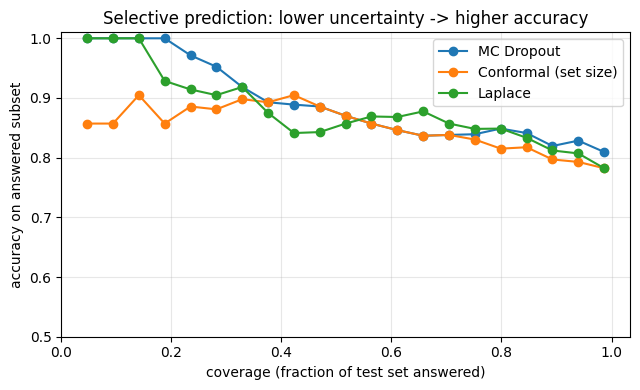
7. Selective prediction with the uncertainty signal

A practical use of any of these scalar uncertainties is selective prediction: refuse to answer when the model is unsure. Sweep a coverage threshold (“only answer on the most-confident X % of the test set”) and watch accuracy improve as we abstain on the noisy tail.

def selective_curve(uncertainty, predictions, y_true):
    """Return (coverage, accuracy) pairs as we abstain on the most-uncertain samples."""
    order = np.argsort(uncertainty)        # most certain first
    y_arr = np.asarray(y_true)
    n = len(order)
    coverages, accuracies = [], []
    for k in range(max(1, n // 20), n + 1, max(1, n // 20)):
        kept = order[:k]
        coverages.append(k / n)
        accuracies.append(float((predictions[kept] == y_arr[kept]).mean()))
    return np.asarray(coverages), np.asarray(accuracies)

fig, ax = plt.subplots(figsize=(6.5, 4))
for label, result in [
    ('MC Dropout', mc_result),
    ('Conformal (set size)', cp_result),
] + ([('Laplace', la_result)] if have_laplace else []):
    cov, acc = selective_curve(result.uncertainty, result.predictions, y_te)
    ax.plot(cov, acc, marker='o', linewidth=1.5, label=label)
ax.set_xlabel('coverage (fraction of test set answered)')
ax.set_ylabel('accuracy on answered subset')
ax.set_title('Selective prediction: lower uncertainty -> higher accuracy')
ax.set_ylim(0.5, 1.01)
ax.legend()
ax.grid(alpha=0.3)
fig.tight_layout()
plt.show()

Recap

All three estimators expose the same predict_with_uncertainty(X) interface and return an UncertaintyResult with predictions, proba_mean, uncertainty, optional epistemic / aleatoric, and method-specific extras under metadata.

Method	Decomposes?	Calibration set?	Extra dependency	Best for
MCDropoutEstimator	epistemic + aleatoric	no	none	Quick uncertainty on a model with dropout.
ConformalPredictor	no	yes	none	Distribution-free coverage guarantees, prediction sets.
LaplaceEstimator	epistemic + aleatoric	yes	laplace-torch	Posterior-based uncertainty without retraining.

See docs/source/api/uncertainty.rst for the full API reference.